Normality Tests
The Normality Tests command performs hypothesis tests to examine whether or not the observations follow a normal distribution. The command performs following hypothesis tests - Kolmogorov-Smirnov (Lilliefors), Shapiro-Wilk W, D'Agostino-Pearson Skewness, Kurtosis and Omnibus K2 tests. Normal probability plot could be produced to graphically assess whether the sample comes from a normal distribution.
How To
Run: Statistics→Basic Statistics→Normality Tests...
Select variables.
Optionally, histogram with normal curve overlay could be plotted for each variable – use the Histogram option in the Advanced Options.
Results
Table with descriptive statistics and hypothesis tests results is produced for each variable.
Sample size, Standard Deviation, Mean, Median, Skewness, Kurtosis, Alternative Skewness (Fisher's), Alternative Kurtosis (Fisher's) - see the Descriptive Statistics procedure for more information.
Null hypothesis H0: The data follow a normal
distribution.
Alternative hypothesis H1: The data do not follow a normal
distribution.
Kolmogorov-Smirnov Test (with Lilliefors correction)
The Kolmogorov-Smirnov test (K-S test) compares sample data with a fitted normal distribution to decide if a sample comes from a population with a normal distribution. Test statistic is defined as
![]() ,
,
where CDF is the normal cumulative distribution function.
When the CDF parameters are not known a priori, the test becomes conservative and loses power. The Lilliefors correction (K-S-L test) of the Kolmogorov-Smirnov test (Lilliefors 1967) estimates the mean and standard deviation of the CDF from the data. The correction uses different critical values and produces more powerful test.
P-value calculation is based on the analytic approximation proposed by Dallal and Wilkinson (1986). If the p-value is less than α (default value – 0.05), the null hypothesis (the distribution is normal) is rejected.
The Kolmogorov-Smirnov/Stephens test is a modification proposed by Stephens (1974). The p-value is based on published critical values and can range only from 0.01 to 0.15 and is provided only for reference.
Shapiro-Wilk W
The Shapiro-Wilk test, proposed by Shapiro in 1965, is considered the most reliable test for non-normality for small to medium sized samples by many authors. The test statistic is defined as:
![]()
Here ![]() is
the ith sample value in ascending order,
is
the ith sample value in ascending order, ![]() is
sample mean and
is
sample mean and ![]() constants
are defined as components of the vector
constants
are defined as components of the vector ![]() , where
, where
![]() are
the expected values of the order statistics of independent and identically distributed
(i.i.d.) random variables sampled from the standard normal
distribution
are
the expected values of the order statistics of independent and identically distributed
(i.i.d.) random variables sampled from the standard normal
distribution![]() , and
V is the covariance matrix of those statistics.
, and
V is the covariance matrix of those statistics.
Anderson–Darling
The Anderson–Darling test checks if a given sample of data is drawn from a specific distribution. The test, proposed by Stephens in 1974, is a modified Kolmogorov-Smirnov test, but gives more weight to the tails of the distribution. The test statistic is defined as:
![]() ,
,
where
![]() ,
, ![]() is
the cumulative distribution function and
is
the cumulative distribution function and ![]() are
the ordered sample values. The better the distribution fits the data, the
smaller is the value of the test statistic.
are
the ordered sample values. The better the distribution fits the data, the
smaller is the value of the test statistic.
D'Agostino Tests
D'Agostino (1970) describes a normality tests
based on the skewness ![]() and
kurtosis
and
kurtosis ![]() coefficients.
For the normal distribution, the theoretical value of skewness is zero, and the
theoretical value of kurtosis is three.
coefficients.
For the normal distribution, the theoretical value of skewness is zero, and the
theoretical value of kurtosis is three.
D'Agostino Skewness
This test is developed to determine if the value of
skewness ![]() is
significantly different from zero.
is
significantly different from zero.
The test statistic is defined as: ![]() where
the values
where
the values ![]() are
defined in the following way:
are
defined in the following way:
![]()
![]()
The test statistic Z(b1) is
approximately normally distributed under the null hypothesis of population normality.
The null hypothesis of normality is rejected if the p-value is less than ![]() level
(0.05).
level
(0.05).
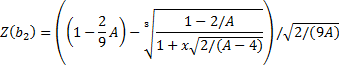
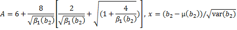
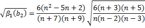
D'Agostino Kurtosis
This test is developed to determine if the
value of kurtosis coefficient ![]() is
significantly different from 3. The test statistic
is
significantly different from 3. The test statistic ![]() is approximately
normally distributed
is approximately
normally distributed ![]() under
the null hypothesis of population normality.
under
the null hypothesis of population normality.
![]()
D'Agostino Omnibus
This test combines ![]() and
and ![]() to produce
an omnibus test of normality. The test statistic
to produce
an omnibus test of normality. The test statistic ![]() is
approximately distributed as a chi-square with two degrees of freedom when the
population is normally distributed.
is
approximately distributed as a chi-square with two degrees of freedom when the
population is normally distributed. ![]() is
defined as
is
defined as
![]() .
.
References
Conover, W. J. (1999). Practical Nonparametric Statistics, Third Edition, New York: John Wiley & Sons.
D’Agostino, R., 1970. Transformation to normality of the null distribution of g1, Biometrika 58, 679–681.
D’Agostino, R., Pearson, E.,
1973. Tests for departures from normality. Empirical results for the
distribution of b1 and b2., Biometrika 60, 613–622.
D’Agostino, R. B., A. J. Belanger, and R. B. D’Agostino, Jr. 1990. A suggestion
for using powerful and informative tests of normality. American Statistician
44: 316–321.
Dallal G.E., Wilkinson L. (1986). An analytic approximation to the distribution of Lilliefors' test for normality. The American Statistician 40: 294–296.
Lilliefors, H. (1967). On the Kolmogorov–Smirnov test for normality with mean and variance unknown, Journal of the American Statistical Association, Vol. 62. pp. 399–402.
Shapiro, S. S.; Wilk, M. B. (1965). An analysis of variance test for normality (complete samples). Biometrika 52 (3–4): 591–611.
Stephens, M. A. (1974). EDF Statistics for Goodness of Fit and Some Comparisons, Journal of the American Statistical Association 69: 730–737.
Thode Jr., H.C. (2002). Testing for Normality. Marcel Dekker, New York.