Linear Correlation (Pearson)
The Linear Correlation (Pearson) command calculates the Pearson product moment correlation coefficient between each pair of variables. Pearson correlation coefficient measures the strength of the linear association between variables.
For ranked data consider using the Spearman's r correlation coefficient (Rank Correlations command).
Assumptions
Each variable should be continuous, random sample and approximately normally distributed.
How To
Run: Statistics→Basic Statistics→Linear Correlation (Pearson)...
Select the variables to correlate.
Pairwise deletion is default for missing values removal (use the Missing values option in the Preferences window to force the casewise deletion).
Results
Matrix with correlation coefficients, critical values and p-values for each pair of variables is produced. The null hypothesis of no linear association is tested for each correlation coefficient. Below the matrix the R-values are listed in order of R absolute value.
Sample size – shows how many cases were used for the calculations. The variables must have the same number of observations (the size of the variable with the least observations count is used).
Critical Value(![]() ) -
) - ![]() critical
value for T-statistic, used to test the null hypothesis.
critical
value for T-statistic, used to test the null hypothesis.
R – Pearson correlation coefficient. For two variables R is defined by
![]()
where ![]() and
and ![]() are the sample standard deviations of X
and Y.
are the sample standard deviations of X
and Y.
The correlation coefficient can take a range of values from +1 to -1. Positive correlation coefficient means that if one variable gets bigger, the other variable also gets bigger, so they tend to move in the same direction. But please note that even strong correlation does not imply causation. Negative correlation coefficient means that the variables tend to move in the opposite directions: If one variable increases, the other variable decreases, and vice-versa. When correlation coefficient is close to zero two variables have no linear relationship.
There are many rules of thumb on how to interpret a correlation coefficient, but all of them are domain specific. For example, here is correlation coefficient interpretation for behavioral sciences offered by Hinkle, Wiersma and Jurs (2003):
|
Absolute value of coefficient |
Strength of correlation |
|
0.90 – 1.00 |
Very high |
|
0.70 – 0.90 |
High |
|
0.50 – 0.70 |
Moderate |
|
0.30 – 0.50 |
Low |
|
0.00 – 0.30 |
Little, if any |
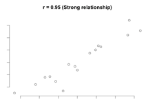
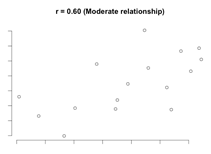
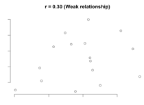
Scatterplots for different correlation coefficients
|
|
|
|
R Standard Error – is the standard error of a correlation coefficient. It is used to determine the confidence intervals around a true correlation of zero. If correlation coefficient is outside of this range, then it is significantly different than zero.
T – is the observed value of
the T-statistic. It is used to test the hypothesis that two variables are
correlated. A T-value near 0 is the evidence for the null hypothesis that there
is no correlation between the variables. When the sample size ![]() is
large, the test statistic
is
large, the test statistic ![]() approximately
follows the Student’s distribution with
approximately
follows the Student’s distribution with ![]() degrees
of freedom.
degrees
of freedom.
p-value – low p-value is
taken as evidence that the null hypothesis can be rejected. The smaller the p-value,
the more significant is linear relationship. If p-value < ![]() we can say
there is a statistically significant relationship between variables.
we can say
there is a statistically significant relationship between variables.
H0 (![]() ) ? – shows if null hypothesis (
) ? – shows if null hypothesis (![]() )
is accepted (written in red) or rejected at
)
is accepted (written in red) or rejected at ![]() (selected
alpha).
(selected
alpha).
References
Hinkle, Wiersma, & Jurs (2003). Applied Statistics for the Behavioral Sciences (5th ed.)